
Storing and analysing larger and larger amounts of data is no longer what drives the decision-making process at successful companies. In today’s world, the key is how fast decision makers are provided with the right information, enabling them to make the right decision before it’s too late.
Streaming analytics help you identify perishable insights, which are the subject of their very own Forrester Report. Perishable insights are results “which must be acted on within a given timeframe or else the chance to influence business outcomes will pass,” according to the IBM Cloud Blog.
The trouble is, many companies see implementing a streaming analytics platform as a very challenging and costly project. This is because, when talking to internal experts or outside consultants, they are usually presented with a very complex architecture – one that needs a lot of effort and money to set up and get going.
That is not the reality of streaming analytics. When the proper set of technologies and tools is used, such a platform can be set up very quickly and effectively.
In facing challenges of this type, I’ve identified a platform that works perfectly. The high-level architecture of this platform is shown below.
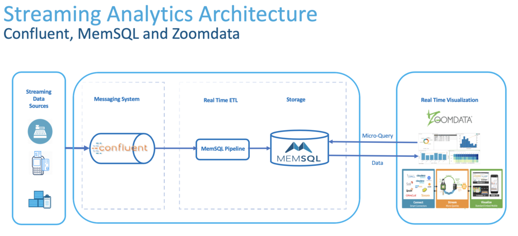
Looks beautiful and simple, doesn’t it? We’re going to use this architecture and build a solution that identifies fraudulent ATM transactions in real time. This platform can solve many other problems as well.) I’ll describe the solution in three steps.
Step 1: Build and Analyze Streams of Data
Everyone in the field of Big Data has heard of Kafka. It’s the backbone of most streaming applications.
Kafka was invented because, for most streaming data, the speed at which the data is generated at the source is a lot faster than the speed at which it can be consumed at the destination. Therefore, a Kafka connection, called a topic, is required to act as a buffer. It receives data from a source, called a publisher, and holds onto it until it’s read by the destination, called a consumer.
Like other streaming solutions, we’re going to use Kafka here as well. But not just any edition of it; we’ll be using Confluent Kafka. Confluent has not only put great add-ons around Kafka, and made it a lot easier to deploy and manage; they are the pioneer in stream processing. Furthermore, Confluent Kafka scales very efficiently, and is able to work very fast, and with very big data, without any hiccups.
The most interesting component in Confluent platform for me is KSQL. It provides a SQL-like querying capability on top of streams of data. And that sounds like heaven for someone like me, who has spent most of his professional life writing and optimizing SQL queries. ]
For the first part of this solution, I followed this blog post and created the streams and processed them with KSQL. The steps I took were:
Download and set up Confluent platform: https://www.confluent.io/download-cp/
Start your Confluent platform:
./bin/confluent startDownload and set up gess: https://github.com/rmoff/gess
Create the topic, using Confluent’s “kafka-topics” command:
./bin/kafka-topics –topic atm_txns –zookeeper localhost:2181 —create –partitions 1 –replication-factor 1Follow the blog post and create and process the stream.
Just as a reference, your final Stream should look like this:
CREATE STREAM ATM_POSSIBLE_FRAUD \
WITH (PARTITIONS=1) AS \
SELECT TIMESTAMPTOSTRING(T1.ROWTIME, ‘yyyy-MM-dd HH:mm:ss’) AS T1_TIMESTAMP, TIMESTAMPTOSTRING(T2.ROWTIME, ‘yyyy-MM-dd HH:mm:ss’) AS T2_TIMESTAMP, \
GEO_DISTANCE(T1.location->lat, T1.location->lon, T2.location->lat, T2.location->lon, ‘KM’) AS DISTANCE_BETWEEN_TXN_KM, \
(T2.ROWTIME – T1.ROWTIME) AS MILLISECONDS_DIFFERENCE, \
(CAST(T2.ROWTIME AS DOUBLE) – CAST(T1.ROWTIME AS DOUBLE)) / 1000 / 60 AS MINUTES_DIFFERENCE, \
GEO_DISTANCE(T1.location->lat, T1.location->lon, T2.location->lat, T2.location->lon, ‘KM’) / ((CAST(T2.ROWTIME AS DOUBLE) – CAST(T1.ROWTIME AS DOUBLE)) / 1000 / 60 / 60) AS KMH_REQUIRED, \
T1.ACCOUNT_ID AS ACCOUNT_ID, \
T1.TRANSACTION_ID, T2.TRANSACTION_ID, \
T1.AMOUNT, T2.AMOUNT, \
T1.ATM, T2.ATM, \
T1.location->lat AS T1_LAT, \
T1.location->lon AS T1_LON, \
T2.location->lat AS T2_LAT, \
T2.location->lon AS T2_LON \
FROM ATM_TXNS T1 \
INNER JOIN ATM_TXNS_02 T2 \
WITHIN (0 MINUTES, 10 MINUTES) \
ON T1.ACCOUNT_ID = T2.ACCOUNT_ID \
WHERE T1.TRANSACTION_ID != T2.TRANSACTION_ID \
AND (T1.location->lat != T2.location->lat OR \
T1.location->lon != T2.location->lon) \
AND T2.ROWTIME != T1.ROWTIME;
Step 2: Ingest Streams of Data into Data Store in Real-Time
The next layer we need to implement in this architecture is data ingestion and storage. There are different tools in the market that are able to ingest data in close to real time, such as Nifi, StreamSets, and maybe Talend. And then for storage, depending on your preference as to on-premise or cloud, HDFS or Object Storage are the options.
The number one factor that I always consider when suggesting a solution to my clients is integrity and homogeneity in all layers of the purpose-built solutions. And when it comes to streaming, where performance is the number one factor, I can’t think of a solution more reliable and faster than SingleStore. If you’re curious to know how fast the database is, watch this video. And be prepared for your mind to be blown!
Another reason I love SingleStore for streaming use cases is how well it integrates with Kafka through SingleStore Pipelines. Take the following steps to set up SingleStore and integrate it with your Confluent platform:
Install SingleStore on the environment of your choice:
https://docs.singlestore.com/db/latest/en/deploy.htmlFire up the SingleStore command-line interface and create a new database:
create database streaming_demo_database;
Create a new table for the records you receive from Confluent:
CREATE TABLE atm_possible_fraud (INGESTION_TIME TIMESTAMP DEFAULT CURRENT_TIMESTAMP ON UPDATE CURRENT_TIMESTAMP
, MESSAGE_FROM_KAFKA JSON
, T1_TIMESTAMP AS MESSAGE_FROM_KAFKA::$T1_TIMESTAMP PERSISTED DATETIME
, T2_TIMESTAMP AS MESSAGE_FROM_KAFKA::$T2_TIMESTAMP PERSISTED DATETIME
, DISTANCE_BETWEEN_TXN_KM AS MESSAGE_FROM_KAFKA::$DISTANCE_BETWEEN_TXN_KM PERSISTED DOUBLE
,MILLISECONDS_DIFFERENCE AS MESSAGE_FROM_KAFKA::$MILLISECONDS_DIFFERENCE PERSISTED DOUBLE
,MINUTES_DIFFERENCE AS MESSAGE_FROM_KAFKA::$MINUTES_DIFFERENCE PERSISTED DOUBLE
,KMH_REQUIRED AS MESSAGE_FROM_KAFKA::$KMH_REQUIRED PERSISTED DOUBLE
,ACCOUNT_ID AS MESSAGE_FROM_KAFKA::$ACCOUNT_ID PERSISTED CHAR(100)
,T1_TRANSACTION_ID AS MESSAGE_FROM_KAFKA::$T1_TRANSACTION_ID PERSISTED CHAR(100)
,T2_TRANSACTION_ID AS MESSAGE_FROM_KAFKA::$T2_TRANSACTION_ID PERSISTED CHAR(100)
,T1_AMOUNT AS MESSAGE_FROM_KAFKA::$T1_AMOUNT PERSISTED DOUBLE
,T2_AMOUNT AS MESSAGE_FROM_KAFKA::$T2_AMOUNT PERSISTED DOUBLE
,T1_ATM AS MESSAGE_FROM_KAFKA::$T1_ATM PERSISTED CHAR(100)
,T2_ATM AS MESSAGE_FROM_KAFKA::$T2_ATM PERSISTED CHAR(100)
,T1_LAT AS MESSAGE_FROM_KAFKA::$T1_LAT PERSISTED DOUBLE
,T1_LON AS MESSAGE_FROM_KAFKA::$T1_LON PERSISTED DOUBLE
,T2_LAT AS MESSAGE_FROM_KAFKA::$T2_LAT PERSISTED DOUBLE
,T2_LON AS MESSAGE_FROM_KAFKA::\$T2_LON PERSISTED DOUBLE
);
Note: A few points about this create table script:
- The first column, INGESTION_TIME, is populated automatically when every record is ingested
- The second column, MESSAGE_FROM_KAFKA, holds the records received from Confluent topics in JSON format
- The rest are Persistent Computed columns in the table that are computed and populated when each JSON record lands in the table. This is another cool feature of SingleStore, makes it incredible easy to parse JSON data without the need to call any additional script or coding.
- Create an index on INGESTION_TIME column. This is needed when we get to build our visualisation work in real-time with Zoomdata:
CREATE INDEX inserttime_index ON atm_possible_fraud (Ingestion_Time);
- Create a pipeline that reads data from Confluent topics and inserts into SingleStore in real-time:
CREATE PIPELINE atm_possible_fraud AS LOAD DATA KAFKA ‘[IP_ADDRESS]:9092/ATM_POSSIBLE_FRAUD’ INTO TABLE atm_possible_fraud (MESSAGE_FROM_KAFKA);
- Test and start the pipeline:
TEST PIPELINE atm_possible_fraud;
START PIPELINE atm_possible_fraud;
And we’re done. Now you can start ingesting data into Confluent Kafka topics and they will be replicated in your SingleStore table in real time.
On your Confluent server, make sure you have started your Confluent platform by running:
./bin/confluent status
Then go to the folder where you have downloaded gess and run following commands:
./gess.sh start
nc -v -u -l 6900 | [CONFLUENT_DIRECTORY]/bin/kafka-console-producer –broker-list localhost:9092 –topic atm_txns
…and start querying your SingleStore table. You should see records ingested in there as they are generated from the source and delivered into the appropriate Kafka topic in Congruent.
Step 3: Visualise Your Data in Real Time
There are so many visualisation tools out there in the market, some of which claim they can visualise your data in real-time. But none of them can truly achieve that. Why? Because they all need to take custody of data to be able to visualise it: each and every record needs to be moved to the server where the visualisation engine runs, processed there, and then visualised to users in the form of graphs and dashboards.
There is one visualisation tool that is different from every other tool in the market, in that it pushes down the query processing to the source where data is stored. That tool is Zoomdata.
Zoomdata doesn’t move data. It doesn’t take custody of the data. How does it work? I’m glad you asked.
Zoomdata’s smart query engine takes the query that is meant to grab the data for the dashboard, applies its knowledge of the underlying data store and metadata about the tables involved in the visualisation, and breaks the query into many smaller queries called micro-queries.
The idea is that, instead of sending a big query down to the source and waiting for the result to come back, it makes more sense to send those smaller queries down, then progressively sharpen the visualisation as the results are returned from each micro-query.
Another very important point about Zoomdata is that it is truly self-service, unlike some other tools, which require a certification to master.
To create a dashboard pointing to the data on our SingleStore database, follow these steps.
Open Zoomdata UI and login as admin.
From the top menu, click on Setting, then select Sources. From installed connectors, click on the SingleStore logo and start configuring the data source.

Give your data source and click Next.
This is the page where you give the details and credentials to connect to your SingleStore cluster. Fill it up and then click Next.
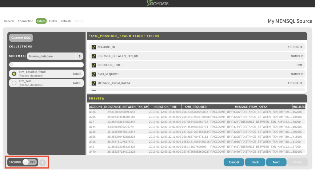
You’ll see the list of tables that exist in the data source you created, in our case the SingleStore database. Select “atm_possible_fraud.”
The list of columns and sample the top 10 rows of the table will be loaded. Remember to toggle CACHING off, since we are building a real time dashboard. Then click Next.
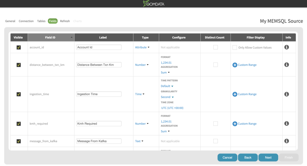
- The next page has the list of columns and their data types. Zoomdata infers the data types for each column from the data source. Change them if they don’t match the type of analysis you want to do, or if they are not correct. Read more about this tab here. After you review the data types for each column, click Next.
The next tab is where you define how often you would like to refresh the cached data. We don’t need to make any changes here since we’re not caching any data. Click Save & Next.
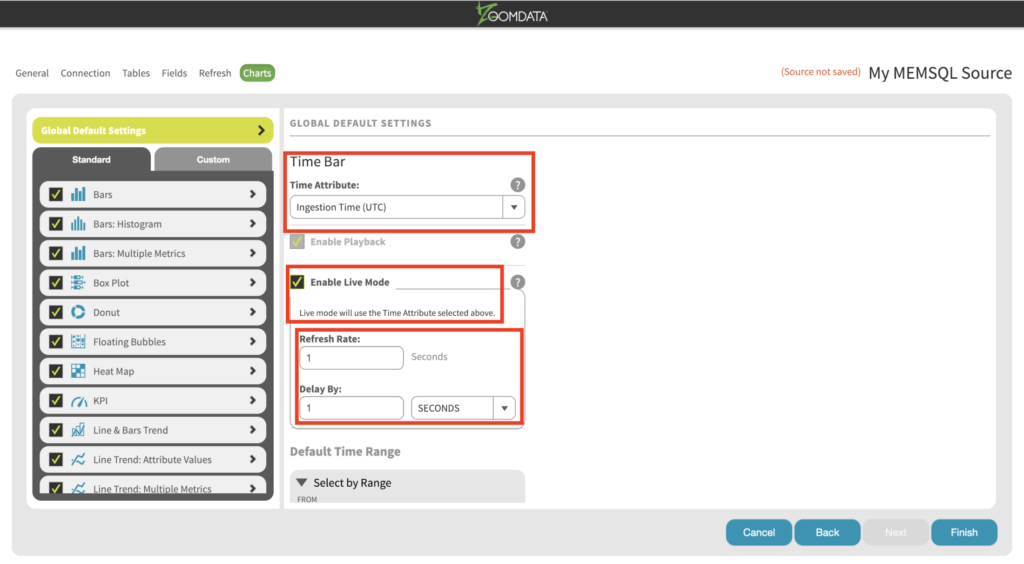
Now we’re on the Charts tab. This tab is used to define the default behaviour of each visualisation type. This means you can define which columns to used to render each visualisation when the dashboard loads. (Zoomdata is 100% self service, meaning that users can change the dashboards at runtime without the need for IT or highly technical resources).
Another very important and interesting feature of your visualisation dashboard will be defined in this tab as well: the Time Bar. Zoomdata follows a streaming architecture, which enables it to connect in “Live Mode” to any data source capable of real-time data. The technology behind this feature is called Data DVR.
In Live Mode, Zoomdata visualisations immediately reflect changes in the source data as data streams in. The live stream can be paused, rewound and replayed, essentially treating it as a digital video recorder (DVR) for your data. Follow these steps to set it up:
- Select Ingestion Time from the Time Attribute drop-down. (That’s the column we had our SingleStore table partitioned by, remember?) This is the column driving our time bar, and it makes sense to choose it: our real-time dashboard needs to be able to get the values from our real-time data source, based on this column, very fast.
- Click the Enable Live Mode checkbox.
- Select 1 for Refresh Rate and 1 second for Delay By. The idea is that Zoomdata will look for records added to the data source with 1 second delay. (In a future version, Zoomdata will be able to support one millisecond delays.)
- Click Finish.
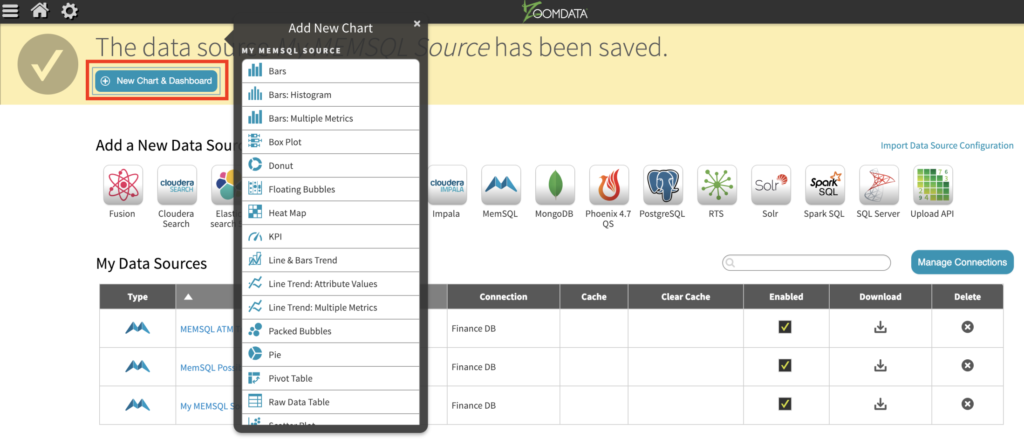
- You will be redirected to the source page. You’ll see on the top that your new data source has been created. Click on New Chart and Dashboard and start building live visualisations.
- Finish visualisations as needed.
Here is a short video showing the incredible performance this streaming solution can provide. On the left side of the video I kick off my script that publishes records to Confluent Kafka topics, and it takes less than three seconds from that point until the visualisation is updated.
Our solution was so simple and easy to implement that I’ve summarized it here in a single blog post. Yet, at the same time, it’s capable of providing incredible performance running on just three servers – one Confluent, one SingleStore, and one Zoomdata.
This post is from Saeed Barghi’s blog, The Business Intelligence Palace. The original version of this post appears on his blog.
Want to know more about any of these products? Reach out to the author at his blog or contact SingleStore.


